My MOOC on Ignorance!

After a year of preparation and hard slog, together with my colleague Gabriele Bammer, I’ve prepared a MOOC (Massive Open Online Course) on Ignorance. The MOOC is based on my work on this topic, and those of you who have followed my blog will find extensions and elaborations of the material covered in my posts. Gabriele’s contributions focus on the roles of ignorance in complex problems.

The course presents a comprehensive framework for understanding, coping with, and making decisions in the face of ignorance. Course participants will learn that ignorance is not always negative, but has uses and benefits in domains ranging from everyday life to the farthest reaches of science where ignorance is simultaneously destroyed and new ignorance created. They will discover the roles ignorance plays in human relationships, culture, institutions, and how it underpins important kinds of social capital.

In addition to video lectures, discussion topics, glossaries, and readings, I’ve provided some html-5 games that give hands-on experience in making decisions in the face of various kinds of unknowns.  The video lectures have captions in Chinese as well as English, and transcripts of the lectures are available in three languages: English, Simplified Chinese and Traditional Chinese. There also are Wiki glossaries for each week in both English and Chinese.

Putting all this together was quite a learning experience for me, and also a dream come true.  I’d come to realize that an interdisciplinary course on ignorance was never going to be a core component of any single discipline’s curriculum, because it doesn’t belong in any one discipline—It sprawls across disciplines.  So a MOOC seems an ideal vehicle for this topic: It’s free and open to everyone. I’ve designed the course to be short enough that other instructors can include it as a component in their own course, and fill the rest of their course with material tailored to their own discipline or profession.

The course will be provided in two five-week blocks. The first one begins on June 23, 2015 and the second on September 22, 2015. There are a lot of MOOCs out there, but there is no other course like this in the world. And ignorance is everyone’s business.  You can watch the promo video here or you can go straight to the registration page here.

 

Impact Factors and the Mismeasure of Quality in Research

Recently Henry Roediger III produced an article in the APA Observer criticizing simplistic uses of Impact Factors (IFs) as measures of research quality. A journal’s IF in a given year is defined as the number of times papers published in the preceding two years have been cited during the given year, divided by the number of papers published in the preceding two years. Roediger’s main points are that IFs involve some basic abuses of statistical and number craft, and they don’t measure what they are being used to measure. He points out that IFs are reported to three decimal places, which usually is spuriously precise. IFs also are means, and yet the citations of papers in most journals are very strongly skewed, with many papers not being cited at all and a few being cited many times. In many such journals the mode and median number of citations per paper both are 0. Finally, he points out that other indicators of impact are ignored, such as whether research publications are used in textbooks or applied in real-world settings. Similar criticisms have been raised in the San Francisco Declaration on Research Assessment, plus the points that IFs can be gamed by editorial policy and that IFs are strongly field-specific.

 

I agree with these points but I don’t think Roediger’s critique goes far enough. The chief problem with IFs is their usage in evaluating individual researchers, research departments, and universities. It should be blindingly obvious that the IF of a journal has almost nothing to do with the number of citations of your or my publications in that journal. The number of citations may be weakly driven by the journal’s reputation and focus, but it also strongly depends on how long your paper has been out there. Citation rates may be a bit more strongly connected with journal IFs than citation totals, but there still are many other factors influencing citation rates. These observations may be obvious, but they seem completely uncomprehended by those who would like to rule academics. Instead, all too often we researchers find ourselves in situations where our fates are being determined by an inappropriate metric that is mindlessly applied by people who know nothing about our research and who lack any modicum of numeracy. The use of IFs for judgments of individual researchers’ output quality should be junked.

 

Number of citations, the h-index, or the i10-index might seem reasonable measures, but there are difficulties with these alternatives too. Young academics can be the victims of the slow accrual of citations.  My own case is a fairly extreme illustration.  My citations currently number more than 2600.  I got my PhD in 1976, so I am about 37 years out of my PhD. Nearly half of those citations (1290) have occurred in the past 5 1/2 years (since 2008). That’s right– 31 years versus less than 6 years for the same number of citations.  In 2012 alone I had approximately 250 citations. This isn’t because I didn’t produce anything of impact until late—Two of my most cited works were published in 1987 and 1989 and have gained about half their citations since 2005 because, frankly, they were ahead of their time. There also seems to be confusion between number of citations and citation-rates. The h and i10 indexes are based on numbers of citations, as is the list of your publications that Google Scholar provides. But the graph of Google Scholar presents of citations of your works by year is presenting information about citation rates. You get a substantially different view of a publication’s impact if you measure it by citations per year since publication than if you do so by total number of citations. For instance, two of my works have nearly identical total numbers of citations (197 and 192), but the first has 7.6 citations/year whereas the second has 19.9 citations/year.  Finally, like IFs, number of citations and citation-rates depend on field-specific characteristics such as the number of people working in your area and achievable publication rates.

   
 

Another thing while I’m on the soap-box: Books should count. My books account for slightly more than half of my citations, and occupy ranks 1, 2, 3, 4, 7, 10, 13, and 14 out of the 75 of my publications that have received any citations. My most widely cited work by a long chalk is a book (published in 1989, now has more than 530 citations, approximately 22 per year, and about half of these since 2005). However, in the Australian science departments, books don’t count. Of course, this isn’t limited to the Australian scene. ISI ignores books and book chapters, and some journals forbid authors to include books or book chapters in their reference lists. This is a purely socially constructed make-believe version of “quality” that sanctions blindness to literature that has real, measurable, and very considerable impact. I have colleagues who seriously consider rewriting highly-cited book chapters and submitting them to journals so that they’ll count. This is sheer make-work of the most wasteful kind.

 

Finally, IFs and citation numbers or rates have no logical connection or demonstrated correlation with the quality of publications. Very bad works can garner high citation rates because numerous authors attack them. Likewise, useful but pedestrian papers can have high citation rates. Conversely, genuinely pioneering works may not be widely cited for a long time. There simply is no substitute for experts making careful assessments of the quality of research publications in their domains of expertise. Numerical indices can help, but they cannot supplant expert judgment. And yet, I claim that this is precisely the attraction that bureaucrats find in single-yardstick numerical measures. They don’t have to know anything about research areas or even basic number-craft to be able to rank-order researchers, departments, and/or entire universities by applying such a yardstick in a perfectly mindless manner. It’s a recipe for us to be ruled and controlled by folk who are massively ignorant and, worse still, meta-ignorant.

 

 

Over-diagnosis and “investigation momentum”

One of my earlier posts, “Making the Wrong Decisions for the Right Reasons”, focused on conditions under which it is futile to pursue greater certainty in the name of better decisions. In this post, I’ll investigate settings in which a highly uncertain outcome should motivate us more strongly than no outcome at all to seek greater certainty. The primary stimulus for this post is a recent letter to JAMA Internal Medicine (Sah, Elias, & Ariely, 2013), entitled “Investigation momentum: the relentless pursuit to resolve uncertainty.” The authors present what they refer to as “another potential downside” to unreliable tests such as prostate-specific antigen (PSA) screening, namely the effect of receiving a “don’t know” result instead of a “positive” or “negative” diagnosis. Their chief claim is that the inconclusive result increases psychological uncertainty which motivates people to seek additional diagnostic testing, whereas untested people would not be motivated to get diagnostic tests. They term this motivation “investigation momentum”, and the obvious metaphor here is that once the juggernaut of testing gets going, it obeys a kind of psychological Newton’s First Law.

The authors’ evidence is an online survey of 727 men aged between 40 and 75 years, with a focus on prostate cancer and PSA screening (e.g., participants were asked to rate their likelihood of developing prostate cancer). The participants were randomly assigned to one of four conditions. In the “no PSA,” condition, participants were given risk information about prostate biopsies. In the other conditions, participants were given information about PSA tests and prostate biopsies. They then were asked to imagine they had just received their PSA test result, which was either “normal”, “elevated”, or “inconclusive”. In the “inconclusive” condition participants were told “This result provides no information about whether or not you have cancer.” After receiving information and (in three conditions) the scenario, participants were asked to indicate whether, considering what they had just been given, they would undergo a biopsy and their level of certainty in that decision.

The study results revealed that, as would be expected, the men whose test result was “elevated” were more likely to say they would get a biopsy than the men in any of the other conditions (61.5% versus 12.7% for those whose result was “normal”, 39.5% for those whose result was “inconclusive”, and 24.5% for those with no PSA). Likewise, the men whose hypothetical result was “normal” were least likely to opt for a biopsy. However, a significantly greater percentage opted for a biopsy if their test was “inconclusive” than those who had no test at all. This latter finding concerned the authors because, as they said, when “tests give no diagnostic information, rationally, from an information perspective, it should be equivalent to never having had the test for the purpose of future decision making.”

Really?

This claim amounts to stating that the patient’s subjective probability of having cancer should remain unchanged after the inconclusive test result. Whether that (rationally) should be the case depends on three things: The patient’s prior subjective probability of having cancer, the patient’s attribution of a probability of cancer to the ambiguous test result, and the relative weights assigned by the patient to the prior and the test result. There are two conditions under which the patient’s prior subjective probability should remain unchanged: (a) The prior subjective probability is identical to the probability attributed to the test, or (b) The test is given a weight of 0. Option (b) seems implausible, so option (a) is the limiting case. Now, it should be clear that if P(cancer|ambiguous test) > P(cancer|prior belief) then P(cancer|prior belief and ambiguous test) > P(cancer|prior belief). Therefore, it could be rational for people to be more inclined to get further tests after an initial test returns an ambiguous result than if they have not yet had any tests.

Let us take one more step. It is plausible that for many people an ambiguous test result would cause them to impute P(cancer|ambiguous test) to be somewhere in the neighbourhood of 1/2. So, for the sake of argument, let’s set P(cancer|ambiguous test) = 1/2. It also is plausible that most people will have an intuitive probability threshold, P_t, beyond which they will be inclined to seek testing. For something as consequential as cancer, we may suppose that for this threshold, P_t < 1/2. Indeed, the authors’ data suggest exactly this. In the no-PSA condition, 16.2% of the men rated their chance of getting prostate cancer above 1/2, but 24.5% of them said they would get a biopsy. Therefore, assuming that all of the 16.2% are included in those who opt for a biopsy, that leaves 8.3% of them in the below-1/2 part of the sample who also opt for a biopsy. An interpolation (see the Technical Bits section below) yields P_t = .38 (group average, of course).

The finding that vexed Sah, et al. is that 39.5% for those whose result was “inconclusive” opted for a biopsy, compared to 24.5% in the no-PSA condition. To begin, let’s assume that the “inconclusive” sample’s P_t also is .38 (after all, the authors find no significant differences among the four samples’ prior probabilities of getting prostate cancer). In the “inconclusive” sample 10.8% rated their chances of getting prostate cancer above 1/2 and 18.9% rated it between .26 and .5. So, our estimate of the percentage whose prior probability is .38 or more is 10.8% + 18.9%/2 = 20.3%. This is the percentage of people in the “inconclusive” sample who would have gone for a biopsy if they had no test, given P_t = .38. That leaves 19.2% to account for in the boost from 20.3% to 39.5% after receiving the inconclusive test result. Now, we can assume that 9.5% are in the .25-.50 range because that’s the total percentage of this sample in that range, so the remaining 9.7% must fall in the 0-.25 range. There are 70.3% altogether in that range, so a linear interpolation gives us a lowest probability for the 9.7% we need to account for of .25 (1 – 9.7/70.3) = .2155.

Now we need to compute the maximum relative weight of the test required to raise a subjective probability of .2155 to the threshold .38. From our formula in the Technical Bits section, we have

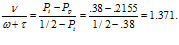
That is, the test would have to be given at most about 1.37 times the weight that each person gives to their own prior subjective probability of prostate cancer. Weighting the test 1.37 times more than one’s prior probability doesn’t seem like giving outlandish weight to the test. And therefore, a plausible case has been put that the tendency for more people to opt for further testing after an inconclusive test result might not be due to psychological “momentum” at all, but instead the product of rational thought. I’m not claiming that the 727 men in the study actually are doing Bayesian calculations—I’m just pointing out that the authors’ findings can be just as readily explained by attributing Bayesian rationality to them as by inferring that they are in the thrall of some kind of psychological “momentum”. The key to understanding all this intuitively is the distinction (introduced by Keynes in 1921) between the weight vs strength (or extremity) of evidence. An inconclusive test is not extreme, i.e., favouring neither the hypothesis that one has the disease or is clear of it. Nevertheless, it still adds its own weight.

Technical Bits

The P_t = .38 result is obtained by a simple linear interpolation. There is 8.3% of the no-PSA sample that fall in the next range below 1/2, which in the authors’ table is a range from .26 to .50. All up, 16% of this sample are in that range, so assuming that the 8.3% are the top-raters in that bunch, our estimate of their lowest probability is .50 – 8.3(.50-.26)/16 = .38.

The relative weight of the test is determined by assuming that the participant is reasoning like a Bayesian agent. Assuming that P(cancer|ambiguous test) = 1/2, we may determine when these conditions could occur for a Bayesian agent whose subjective probability, P(cancer|prior belief) , has a Beta() distribution and therefore a mean of . To begin, the first condition would be satisfied if  > P_t. Now denoting the relative weight of the test by , the posterior distribution of P(cancer|prior belief and ambiguous test) would be Beta(). So, the second condition would be satisfied if  > P_t. Solving for the weight, we get


This makes intuitive sense in two respects. First, the numerator is positive only if  < P_t, i.e., if the first condition hasn’t already been satisfied. The further  is below P_t, the greater the weight needs to be in order for the above inequality to be satisfied. Second, the denominator tells us that the further P_t is below ½, the less weight needs to be given to the test for that inequality to be satisfied.

The “precision” of a Beta() distribution is . The greater this sum, the tighter the distribution is around its mean. So the precision can be used as a proxy for the weight of evidence associated by an agent to their prior belief. The test adds to the precision because it is additional evidence: So now we can compare the weight of the test relative to the precision of the prior: Given the minimal weight required in the previous equation, we get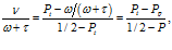


where P_p is the agent’s mean prior probability of getting cancer.

 

 

 

Digital “poster” and Integration and Implementation Sciences Conference

I’ll indulge in a bit more shameless advertising here, but it’s directly relevant to this blog. First, I’m one among several plenary speakers at what’s billed as the First Global Conference on Research Integration and Implementation (8-11 September). As the entry webpage says, the main goal is bringing together everyone whose research interests include:

• understanding problems as systems,
• combining knowledge from various disciplines and practice areas,
• dealing with unknowns to reduce risk, unpleasant surprises and adverse unintended consequences,
• helping research teams collaborate more effectively, and
• implementing evidence in improved policy and practice.

Although the physical conference takes place in Canberra, Australia, we have an extensive online conference setup and co-conferences taking place in Germany, The Netherlands, and Uruguay. Most of the conference will be broadcast live over the net.

In addition to the information about the program, participants, and events, you can get a fair idea of what the conference is about by browsing the digital posters. So this is where the shameless advert comes in. My digital poster is essentially a couple of slides of links describing my thinking about ignorance, uncertainty and the unknown over the past 25 years or so. The links go to my publications, posts on this blog, and works by others on this topic. You can get to my poster is by scrolling down this list and clicking the relevant link.

A Few (More) Myths about “Big Data”

Following on from Kate Crawford’s recent and excellent elaboration of six myths about “big data”, I should like to add four more that highlight important issues about such data that can misguide us if we ignore them or are ignorant of them.

Myth 7: Big data are precise.

As with analyses of almost any other kind of data, big data analyses largely consists of estimates. Often these estimates are based on sample data rather than population data, and the samples may not be representative of their referent populations (as Crawford points out, but also see Myth 8). Moreover, big data are even less likely than “ordinary” data to be free of recording errors or deliberate falsification.

Even when the samples are good and the sample data are accurately recorded, estimates still are merely estimates, and the most common mistake decision makers and other stakeholders make about estimates is treating them as if they are precise or exact. In a 1990 paper I referred to this as the fallacy of false precision. Estimates always are imprecise, and ignoring how imprecise they are is equivalent to ignoring how wrong they could be. Major polling companies gradually learned to report confidence intervals or error-rates along with their estimates and to take these seriously, but most government departments apparently have yet to grasp this obvious truth.

Why might estimate error be a greater problem for big data than for “ordinary” data? There are at least two reasons. First, it is likely to be more difficult to verify the integrity or veracity of big data simply because it is integrated from numerous sources. Second, if big datasets are constructed from multiple sources, each consisting of an estimate with its own imprecision, then these imprecisions may propagate. To give a brief illustration, if estimate X has variance _x², estimate Y has variance _y², X and Y are independent of one another, and our “big” dataset consists of adding X+Y to get Z, then the variance of Z will be _x² + _y².

Myth 8: Big data are accurate.

There are two senses in which big data may be inaccurate, in addition to random variability (i.e., sampling error): Biases, and measurement confounds. Economic indicators of such things as unemployment rates, inflation, or GDP in most countries are biased. The bias stems from the “shadow” (off the books) economic activity in most countries. There is little evidence that economic policy makers in most countries pay any attention to such distortions when using economic indicators to inform policies.

Measurement confounds are a somewhat more subtle issue, but the main idea is that data may not measure what we think it is measuring because it is influenced by extraneous factors. Economic indicators are, again, good examples but there are plenty of others (don’t get me started on the idiotic bibliometrics and other KPIs that are imposed on us academics in the name of “performance” assessment). Web analytics experts are just beginning to face up to this problem. For instance, webpage dwell times are not just influenced by how interested the visitor is in the content of a webpage, but may also reflect such things as how difficult the contents are to understand, the visitor’s attention span, or the fact that they left their browsing device to do something else and then returned much later. As in Myth 7, bias and measurement confounds may be compounded in big data to a greater extent than they are in small data, simply because big data often combines multiple measures.

Myth 9. Big data are stable.

Data often are not recorded just once, but re-recorded as better information becomes available or as errors are discovered. In a recent Wall Street Journal article, economist Samuel Rines presented several illustrations of how unstable economic indicator estimates are in the U.S. For example, he observed that in November 2012 the first official estimate of net employment increase was 146,000 new jobs. By the third revision that number had increased by 68% to 247,000. In another instance, he pointed out that American GDP annual estimates each year typically are revised several times, and often substantially, as the year slides into the past.

Again, there is little evidence that people crafting policy or making decisions based on these numbers take their inherent instability into account. One may protest that often decisions must be made before “final” revisions can be completed. However, where such revisions in the past have been recorded, the degree of instability in these indicators should not be difficult to estimate. These could be taken into account, at the very least, in worst- and best-case scenario generation.

Myth 10. We have adequate computing power and techniques to analyse big data.

Analysing big data is a computationally intense undertaking, and at least some worthwhile analytical goals are beyond our reach, in terms of computing power and even, in some cases, techniques. I’ll give just one example. Suppose we want to model the total dwell time per session of a typical user who is browsing the web. The number of items on which the user dwells is a random variable, and so is the amount of dwell time for each item. The total dwell time, then, is what is called a “randomly stopped sum”. The expression for the probability distribution of a randomly stopped sum doesn’t have a closed form (it’s an infinite sum), so it can’t be modelled via conventional statistical estimation techniques (least-squares or maximum likelihood). Instead, there are two viable approaches: Simulation and Bayesian hierarchical MCMC. I’m writing a paper on this topic, and from my own experience I can declare that either technique would require a super-computer for datasets of the kind dealt with, e.g., by NRS PADD.

A Book Ate My Blog

Sad, but true—I’ve been off blogging since late 2011 because I was writing a book (with Ed Merkle) under a contract with Chapman and Hall. Writing the book took up the time I could devote to writing blog posts. Anyhow, I’m back in the blogosophere, and for those unusual people out there who have interests in multivariate statistical modelling, you can find out about the book here or here.

Statistical Significance On Trial

There is a long-running love-hate relationship between the legal and statistical professions, and two vivid examples of this have surfaced in recent news stories, one situated in a court of appeal in London and the other in the U.S. Supreme Court. Briefly, the London judge ruled that Bayes’ theorem must not be used in evidence unless the underlying statistics are “firm;” while the U.S. Supreme Court unanimously ruled that a drug company’s non-disclosure of adverse side-effects cannot be justified by an appeal to the statistical non-significance of those effects. Each case, in its own way, shows why it is high time to find a way to establish an effective rapprochement between these two professions.

The Supreme Court decision has been applauded by statisticians, whereas the London decision has appalled statisticians of similar stripe. Both decisions require some unpacking to understand why statisticians would cheer one and boo the other, and why these are important decisions not only for both the statistical and legal professions but for other domains and disciplines whose practices hinge on legal and statistical codes and frameworks.

This post focuses on the Supreme Court decision. The culprit was a homoeopathic zinc-based medicine, Zicam, manufactured by Matrixx Initivatives, Inc. and advertised as a remedy for the common cold. Matrixx ignored reports from users and doctors since 1999 that Zicam caused some users to experience burning sensations or even to lose the sense of smell. When this story was aired by a doctor on Good Morning America in 2004, Matrixx stock price plummeted.

The company’s defense was that these side-effects were “not statistically significant.” In the ensuing fallout, Matrixx was faced with more than 200 lawsuits by Zicam users, but the case in point here is Siracusano vs Matrixx, in which Mr. Siracusano was suing on behalf of investors on grounds that they had been misled. After a few iterations through the American court system, the question that the Supreme Court ruled on was whether a claim of securities fraud is valid against a company that neglected to warn consumers about effects that had been found to be statistically non-significant. As insider-knowledgeable Stephen Ziliak’s insightful essay points out, the decision will affect drug supply regulation, securities regulation, liability and the nature of adverse side-effects disclosed by drug companies. Ziliak was one of the “friends of the court” providing expert advice on the case.

A key point in this dispute is whether statistical nonsignificance can be used to infer that a potential side-effect is, for practical purposes, no more likely to occur when using the medicine than when not. Among statisticians it is a commonplace that such inferences are illogical (and illegitimate). There are several reasons for this, but I’ll review just two here.

These reasons have to do with common misinterpretations of the measure of statistical significance. Suppose Matrixx had conducted a properly randomized double-blind experiment comparing Zicam-using subjects with those using an indistinguishable placebo, and observed the difference in side-effect rates between the two groups of subjects. One has to bear in mind that random assignment of subjects to one group or the other doesn’t guarantee equivalence between the groups. So, it’s possible that even if there really is no difference between Zicam and the placebo regarding the side-effect, a difference between the groups might occur by “luck of the draw.”

The indicator of statistical significance in this context would be the probability of observing a difference at least as large as the one found in the study if the hypothesis of no difference were true. If this probability is found to be very low (typically .05 or less) then the experimenters will reject the no-difference hypothesis on the grounds that the data they’ve observed would be very unlikely to occur if that hypothesis were true. They will then declare that there is a statistically significant difference between the Zicam and placebo groups. If this probability is not sufficiently low (i.e., greater than .05) the experimenters will decide not to reject the no-difference hypothesis and announce that the difference they found was statistically non-significant.

So the first reason for concern is that Matrixx acted as if statistical nonsignificance entitles one to believe in the hypothesis of no-difference. However, failing to reject the hypothesis of no difference doesn’t entitle one to believe in it. It’s still possible that a difference might exist and the experiment failed to find it because it didn’t have enough subjects or because the experimenters were “unlucky.” Matrixx has plenty of company in committing this error; I know plenty of seasoned researchers who do the same, and I’ve already canvassed the well-known bias in fields such as psychology not to publish experiments that failed to find significant effects.

The second problem arises from a common intuition that the probability of observing a difference at least as large as the one found in the study if the hypothesis of no difference were true tells us something about the inverse—the probability that the no-difference hypothesis is true if we find a difference at least as large as the one observed in our study, or, worse still, the probability that the no-difference hypothesis is true. However, the first probability on its own tells us nothing about the other two.

For a quick intuitive, if fanciful, example let’s imagine randomly sampling one person from the world’s population and our hypothesis is that s/he will be Australian. On randomly selecting our person, all that we know about her initially is that she speaks English.

There are about 750 million first-or second-language English speakers world-wide, and about 23 million Australians. Of the 23 million Australians, about 21 million of them fit the first- or second-language English description. Given that our person speaks English, how likely is it that we’ve found an Australian? The probability that we’ve found an Australian given that we’ve picked an English-speaker is 21/750 = .03. So there goes our hypothesis. However, had we picked an Australian (i.e., given that our hypothesis were true), the probability that s/he speaks English is 21/23 = .91.

See also Ziliak and McCloskey’s 2008 book, which mounts a swinging demolition of the unquestioned application of statistical significance in a variety of domains.

Aside from the judgment about statistical nonsignificance, the most important stipulation of the Supreme Court’s decision is that “something more” is required before a drug company can justifiably decide to not disclose a drug’s potential side-effects. What should this “something more” be? This sounds as if it would need judgments about the “importance” of the side-effects, which could open multiple cans of worms (e.g., Which criteria for importance? According to what or whose standards?). Alternatively, why not simply require drug companies to report all occurrences of adverse side-effects and include the best current estimates of their rates among the population of users?

A slightly larger-picture view of the Matrixx defense resonates with something that I’ve observed in even the best and brightest of my students and colleagues (oh, and me too). And that is the hope that somehow probability or statistical theories will get us off the hook when it comes to making judgments and decisions in the face of uncertainty. It can’t and won’t, especially when it comes to matters of medical, clinical, personal, political, economic, moral, aesthetic, and all the other important kinds of importance.

Scientists on Trial: Risk Communication Becomes Riskier

Back in late May 2011, there were news stories of charges of manslaughter laid against six earthquake experts and a government advisor responsible for evaluating the threat of natural disasters in Italy, on grounds that they allegedly failed to give sufficient warning about the devastating L’Aquila earthquake in 2009. In addition, plaintiffs in a separate civil case are seeking damages in the order of €22.5 million (US$31.6 million). The first hearing of the criminal trial occurred on Tuesday the 20^th of September, and the second session is scheduled for October 1^st.

According to Judge Giuseppe Romano Gargarella, the defendants gave inexact, incomplete and contradictory information about whether smaller tremors in L’Aquila six months before the 6.3 magnitude quake on 6 April, which killed 308 people, were to be considered warning signs of the quake that eventuated. L’Aquila was largely flattened, and thousands of survivors lived in tent camps or temporary housing for months.

If convicted, the defendants face up to 15 years in jail and almost certainly will suffer career-ending consequences. While manslaughter charges for natural disasters have precedents in Italy, they have previously concerned breaches of building codes in quake-prone areas. Interestingly, no action has yet been taken against the engineers who designed the buildings that collapsed, or government officials responsible for enforcing building code compliance. However, there have been indications of lax building codes and the possibility of local corruption.

The trial has, naturally, outraged scientists and others sympathetic to the plight of the earthquake experts. An open letter by the Istituto Nazionale di Geofisica e Vulcanologia (National Institute of Geophysics and Volcanology) said the allegations were unfounded and amounted to “prosecuting scientists for failing to do something they cannot do yet — predict earthquakes”. The AAAS has presented a similar letter, which can be read here.

In pre-trial statements, the defence lawyers also have argued that it was impossible to predict earthquakes. “As we all know, quakes aren’t predictable,” said Marcello Melandri, defence lawyer for defendant Enzo Boschi, who was president of Italy’s National Institute of Geophysics and Volcanology). The implication is that because quakes cannot be predicted, the accusations that the commission’s scientists and civil protection experts should have warned that a major quake was imminent are baseless.

Unfortunately, the Istituto Nazionale di Geofisica e Vulcanologia, the AAAS, and the defence lawyers were missing the point. It seems that failure to predict quakes is not the substance of the accusations. Instead, it is poor communication of the risks, inappropriate reassurance of the local population and inadequate hazard assessment. Contrary to earlier reports, the prosecution apparently is not claiming the earthquake should have been predicted. Instead, their focus is on the nature of the risk messages and advice issued by the experts to the public.

Examples raised by the prosecution include a memo issued after a commission meeting on 31 March 2009 stating that a major quake was “improbable,” a statement to local media that six months of low-magnitude tremors was not unusual in the highly seismic region and did not mean a major quake would follow, and an apparent discounting of the notion that the public should be worried. Against this, defence lawyer Melandri has been reported saying that the panel “never said, ‘stay calm, there is no risk'”.

It is at this point that the issues become both complex (by their nature) and complicated (by people). Several commentators have pointed out that the scientists are distinguished experts, by way of asserting that they are unlikely to have erred in their judgement of the risks. But they are being accused of “incomplete, imprecise, and contradictory information” communication to the public. As one of the civil parties to the lawsuit put it, “Either they didn’t know certain things, which is a problem, or they didn’t know how to communicate what they did know, which is also a problem.”

So, the experts’ scientific expertise is not on trial. Instead, it is their expertise in risk communication. As Stephen S. Hall’s excellent essay in Nature points out, regardless of the outcome this trial is likely to make many scientists more reluctant to engage with the public or the media about risk assessments of all kinds. The AAAS letter makes this point too. And regardless of which country you live in, it is unwise to think “Well, that’s Italy for you. It can’t happen here.” It most certainly can and probably will.

Matters are further complicated by the abnormal nature of the commission meeting on the 31^st of March at a local government office in L’Aquila. Boschi claims that these proceedings normally are closed whereas this meeting was open to government officials, and he and the other scientists at the meeting did not realize that the officials’ agenda was to calm the public. The commission did not issue its usual formal statement, and the minutes of the meeting were not completed, until after the earthquake had occurred. Instead, two members of the commission, Franco Barberi and Bernardo De Bernardinis, along with the mayor and an official from Abruzzo’s civil-protection department, held a now (in)famous press conference after the meeting where they issued reassuring messages.

De Bernardinis, an expert on floods but not earthquakes, incorrectly stated that the numerous earthquakes of the swarm would lessen the risk of a larger earthquake by releasing stress. He also agreed with a journalist’s suggestion that residents enjoy a glass of wine instead of worrying about an impending quake.

The prosecution also is arguing that the commission should have reminded residents in L’Aquila of the fragility of many older buildings, advised them to make preparations for a quake, and reminded them of what to do in the event of a quake. This amounts to an accusation of a failure to perform a duty of care, a duty that many scientists providing risk assessments may dispute that they bear.

After all, telling the public what they should or should not do is a civil or governmental matter, not a scientific one. Thomas Jordan’s essay in New Scientist brings in this verdict: “I can see no merit in prosecuting public servants who were trying in good faith to protect the public under chaotic circumstances. With hindsight their failure to highlight the hazard may be regrettable, but the inactions of a stressed risk-advisory system can hardly be construed as criminal acts on the part of individual scientists.” As Jordan points out, there is a need to separate the role of science advisors from that of civil decision-makers who must weigh the benefits of protective actions against the costs of false alarms. This would seem to be a key issue that urgently needs to be worked through, given the need for scientific input into decisions about extreme hazards and events, both natural and human-caused.

Scientists generally are not trained in communication or in dealing with the media, and communication about risks is an especially tricky undertaking. I would venture to say that the prosecution, defence, judge, and journalists reporting on the trial will not be experts in risk communication either. The problems in risk communication are well known to psychologists and social scientists specializing in its study, but not to non-specialists. Moreover, these specialists will tell you that solutions to those problems are hard to come by.

For example, Otway and Wynne (1989) observed in a classic paper that an “effective” risk message has to simultaneously reassure by saying the risk is tolerable and panic will not help, and warn by stating what actions need to be taken should an emergency arise. They coined the term “reassurance arousal paradox” to describe this tradeoff (which of course is not a paradox, but a tradeoff). The appropriate balance is difficult to achieve, and is made even more so by the fact that not everyone responds in the same way to the same risk message.

It is also well known that laypeople do not think of risks in the same way as risk experts (for instance, laypeople tend to see “hazard” and “risk” as synonyms), nor do they rate risk severity in line with the product of probability and magnitude of consequence, nor do they understand probability—especially low probabilities. Given all of this, it will be interesting to see how the prosecution attempts to establish that the commission’s risk communications contained “incomplete, imprecise, and contradictory information.”

Scientists who try to communicate risks are aware of some of these issues, but usually (and understandably) uninformed about the psychology of risk perception (see, for instance, my posts here and here on communicating uncertainty about climate science). I’ll close with just one example. A recent International Commission on Earthquake Forecasting (ICEF) report argues that frequently updated hazard probabilities are the best way to communicate risk information to the public. Jordan, chair of the ICEF, recommends that “Seismic weather reports, if you will, should be put out on a daily basis.” Laudable as this prescription is, there are at least three problems with it.

Weather reports with probabilities of rain typically present probabilities neither close to 0 nor to 1. Moreover, they usually are anchored on tenths (e.g., .2, or .6 but not precise numbers like .23162 or .62947). Most people have reasonable intuitions about mid-range probabilities such as .2 or .6. But earthquake forecasting has very low probabilities, as was the case in the lead-up to the L’Aquila event. Italian seismologists had estimated the probability of a large earthquake in the next three days had increased from 1 in 200,000, before the earthquake swarm began, to 1 in 1,000 following the two large tremors the day before the quake.

The first problem arises from the small magnitude of these probabilities. Because people are limited in their ability to comprehend and evaluate extreme probabilities, highly unlikely events usually are either ignored or overweighted. The tendency to ignore low-probability events has been cited to account for the well-established phenomenon that homeowners tend to be under-insured against low probability hazards (e.g., earthquake, flood and hurricane damage) in areas prone to those hazards. On the other hand, the tendency to over-weight low-probability events has been used to explain the same people’s propensity to purchase lottery tickets. The point is that low-probability events either excite people out of proportion to their likelihood or fail to excite them altogether.

The second problem is in understanding the increase in risk from 1 in 200,000 to 1 in 1,000. Most people are readily able to comprehend the differences between mid-range probabilities such as an increase in the chance of rain from .2 to .6. However, they may not appreciate the magnitude of the difference between the two low probabilities in our example. For instance, an experimental study with jurors in mock trials found that although DNA evidence is typically expressed in terms of probability (specifically, the probability that the DNA sample could have come from a randomly selected person in the population), jurors were equally likely to convict on the basis of a probability of 1 in 1,000 as a probability of 1 in 1 billion. At the very least, the public would need some training and accustoming to miniscule probabilities.

All this leads us to the third problem. Otway and Wynne’s “reassurance arousal paradox” is exacerbated by risk communications about extremely low-probability hazards, no matter how carefully they are crafted. Recipients of such messages will be highly suggestible, especially when the stakes are high. So, what should the threshold probability be for determining when a “don’t ignore this” message is issued? It can’t be the imbecilic Dick Cheney zero-risk threshold for terrorism threats, but what should it be instead?

Note that this is a matter for policy-makers to decide, not scientists, even though scientific input regarding potential consequences of false alarms and false reassurances should be taken into account. Criminal trials and civil lawsuits punishing the bearers of false reassurances will drive risk communicators to lower their own alarm thresholds, thereby ensuring that they will sound false alarms increasingly often (see my post about making the “wrong” decision most of the time for the “right” reasons).

Risk communication regarding low-probability, high-stakes hazards is one of the most difficult kinds of communication to perform effectively, and most of its problems remain unsolved. The L’Aquila trial probably will have an inhibitory impact on scientists’ willingness to front the media or the public. But it may also stimulate scientists and decision-makers to work together for the resolution of these problems.

The Stapel Case and Data Fabrication

By now it’s all over the net (e.g., here) and international news media: Tilburg University sacked high-profile social psychologist Diederik Stapel, after he was outed as having faked data in his research. Stapel was director of the Tilburg Institute for Behavioral Economics Research, a successful researcher and fundraiser, and as a colleague expressed it, “the poster boy of Dutch social psychology.” He had more than 100 papers published, some in the flagship journals not just of psychology but of science generally (e.g., Science), and won prestigious awards for his research on social cognition and stereotyping.

Tilburg University Rector Philip Eijlander said that Stapel had admitted to using faked data, apparently after Eijlander confronted him with allegations by graduate student research assistants that his research conduct was fraudulent. The story goes that the assistants had identified evidence of data entry by Stapel via copy-and-paste.

Willem Levelt, psycholinguist and former president of the Royal Netherlands Academy of Arts and Sciences, is to lead a panel investigating the extent of the fraud. That extent could be very widespread indeed. In a press conference the Tilburg rector made it clear that Stapel’s fraudulent research practices may have ranged over a number of years. All of his papers would be suspected, and the panel will advise on which papers will have to be retracted. Likewise, the editors of all journals that Stapel published in are also investigating details of his papers that were published in these journals. Then there are Stapel’s own students and research collaborators, whose data and careers may have been contaminated by his.

I feel sorry for my social psychological colleagues, who are reeling in shock and dismay. Some of my closest colleagues knew Stapel (one was a fellow graduate student with him), and none of them suspected him. Among those who knew him well and worked with him, Stapel apparently was respected as a researcher and trusted as a man of integrity. They are asking themselves how his cheating could have gone undetected for so long, and how such deeds could be prevented in the future. They fear its impact on public perception of their discipline and trust in scientific researchers generally.

An understandable knee-jerk reaction is to call for stricter regulation of scientific research, and alterations to the training of researchers. Mark Van Vugt and Anjana Ahuja’s blog post exemplifies this reaction, when they essentially accuse social psychologists of being more likely to engage in fraudulent research because some of them use deception of subjects in their experiments:

“…this means that junior social psychologists are being trained to deceive people and this might be a first violation of scientific integrity. It would be good to have a frank discussion about deception in our discipline. It is not being tolerated elsewhere so why should it be in our field.”

They make several recommendations for reform, including the declaration that “… ultimately it is through training our psychology students into doing ethically sound research that we can tackle scientific fraud. This is no easy feat.”

The most obvious problems with Van Vugt’s and Ahuja’s recommendations are, first, that there is no clear connection between using deception in research designs and faking data, and second, many psychology departments already include research ethics in researcher education and training. Stapel isn’t ignorant of research ethics. But a deeper problem is that none of their recommendations and, thus far, very few of the comments I have seen about this or similar cases, address three of the main considerations in any criminal case: Means, opportunity, and motive.

Let me speak to means and opportunity first. Attempts to more strictly regulate the conduct of scientific research are very unlikely to prevent data fakery, for the simple reason that it’s extremely easy to do in a manner that is extraordinarily difficult to detect. Many of us “fake data” on a regular basis when we run simulations. Indeed, simulating from the posterior distribution is part and parcel of Bayesian statistical inference. It would be (and probably has been) child’s play to add fake cases to one’s data by simulating from the posterior and then jittering them randomly to ensure that the false cases look like real data. Or, if you want to fake data from scratch, there is plenty of freely available code for randomly generating multivariate data with user-chosen probability distributions, means, standard deviations, and correlational structure. So, the means and opportunities are on hand for virtually all of us. They are the very same means that underpin a great deal of (honest) research. It is impossible to prevent data fraud by these means through conventional regulatory mechanisms.

Now let us turn to motive. The most obvious and comforting explanations of cheats like psychologists Stapel or Hauser, or plagiarists like statistician Wegman and political scientist Fischer, are those appealing to their personalities. This is the “X cheated because X is psychopathic” explanation. It’s comforting because it lets the rest of us off the hook (“I wouldn’t cheat because I’m not a psychopath”). Unfortunately this kind of explanation is very likely to be wrong. Most of us cheat on something somewhere along the line. Cheating is rife, for example, among undergraduate university students (among whom are our future researchers!), so psychopathy certainly cannot be the deciding factor there. What else could be the motivational culprit? How about the competitive pressures on researchers generated by the contemporary research culture?

Cognitive psychologist E,J, Wagenmakers (as quoted in Andrew Gelman’s thoughtful recent post) is among the few thus far who have addressed possible motivating factors inherent in the present-day research climate. He points out that social psychology has become very competitive, and

“high-impact publications are only possible for results that are really surprising. Unfortunately, most surprising hypotheses are wrong. That is, unless you test them against data you’ve created yourself. There is a slippery slope here though; although very few researchers will go as far as to make up their own data, many will “torture the data until they confess”, and forget to mention that the results were obtained by torture….”

I would add to E.J.’s observations the following points.

First, social psychology journals (and journals for other areas in psychology) exhibit a strong bias towards publishing only studies that have achieved a statistically significant result. This bias is widely believed in by researchers and their students. The obvious temptation arising from this is to ease an inconclusive finding into being conclusive by adding more “favorable” cases or making some of the unfavorable ones more favorable.

Second, and of course readers will recognize one of my hobby-horses here, the addiction in psychology to hypothesis-testing over parameter estimation amounts to an insistence that every study yield a conclusion or decision: Did the null hypothesis get rejected? The obvious remedy for this is to develop a publication climate that does not insist that each and every study be “conclusive,” but instead emphasizes the importance of a cumulative science built on multiple independent studies, careful parameter estimates and multiple tests of candidate theories. This adds an ethical and motivational rationale to calls for a shift to Bayesian methods in psychology.

Third, journal editors and reviewers routinely insist on more than one study to an article. On the surface, this looks like what I’ve just asked for, a healthy insistence on independent replication. It isn’t, for two reasons. First, even if the multiple studies are replications, they aren’t independent because they come from the same authors and/or lab. Genuinely independent replicated studies would be published in separate papers written by non-overlapping sets of authors from separate labs. However, genuinely independent replication earns no kudos and therefore is uncommon (not just in psychology, either—other sciences suffer from this problem, including those that used to have a tradition of independent replication).

The second reason is that journal editors don’t merely insist on study replications, they also favor studies that come up with “consistent” rather than “inconsistent” findings (i.e., privileging “successful” replications over “failed” replications). By insisting on multiple studies that reproduce the original findings, journal editors are tempting researchers into corner-cutting or outright fraud in the name of ensuring that that first study’s findings actually get replicated. E.J.’s observation that surprising hypotheses are unlikely to be supported by data goes double (squared, actually) when it comes to replication—Support for a surprising hypothesis may occur once in a while, but it is unlikely to occur twice in a row. Again, remedies are obvious: Develop a publication climate which encourages or even insists on independent replication, that treats well-conducted “failed” replications identically to well-conducted “successful” ones, and which does not privilege “replications” from the same authors or lab of the original study.

None of this is meant to say I fall for cultural determinism—Most researchers face the pressures and motivations described above, but few cheat. So personality factors may also exert an influence, along with circumstances specific to those of us who give in to the temptations of cheating. Nevertheless if we want to prevent more Stapels, we’ll get farther by changing the research culture and its motivational effects than we will by exhorting researchers to be good or lecturing them about ethical principles of which they’re already well aware. And we’ll get much farther than we would in a futile attempt to place the collection and entry of every single datum under surveillance by some Stasi-for-scientists.

An Ignorance Economy?

It’s coming up to a year since I began this blog. In my usual fashion, I set myself the unrealistic goal of writing a post every week. This is only the 37^th, so I’ve fallen short by a considerable margin. On the other hand, most of those posts have been on the order of 1500 words long, for a total of about 55,500 words thus far. That seems a fair whack of the keyboard, and it’s been fun too.

In an earlier post I proposed that because of the ways in which knowledge economies work, we increasingly live in an “ignorance society.” In the same year that Sheldon Ungar’s paper on ignorance as a public problem appeared, another paper came out by Joanne Roberts and John Armitage with the intriguing title “The Ignorance Economy.” Their stated purpose was to critique the notion of a knowledge economy via an investigation of ignorance from an economic standpoint.

As Roberts and Armitage (and many others) have said, knowledge as a commodity has several distinctive features. Once knowledge is consumed, it does not disappear and indeed its consumption may result in the development of more knowledge. The consumption of knowledge is non-zero-sum and can be non-excludable. Knowledge is a multiplier resource in this sense. Finally, knowledge is not subject to diminishing returns.

Interestingly, Roberts and Armitage do not say anything substantial about ignorance as a commodity. We already have some characterizations handy from this blog and elsewhere. Like knowledge, ignorance can be non-zero-sum and non-excludable in the sense that my being ignorant about X doesn’t prevent you from also being ignorant about X, nor does greater ignorance on my part necessarily decrease your ignorance. Ignorance also does not seem susceptible to diminishing returns. And of course, new knowledge can generate ignorance, and an important aspect of an effective knowledge-based economy is its capacity for identifying and clarifying unknowns. Even in a booming knowledge economy, ignorance can be a growth industry in its own right.

There are obvious examples of economies that could, in some sense, be called “ignorance economies.” Education and training are ignorance economies in the sense that educators and trainers make their living via a continual supply of ignoramuses who are willing to pay for the privilege of shedding that status. Likewise, governmental and corporate organizations paying knowledge experts enable those experts to make a living out of selling their expertise to those who lack it. This is simply the “underbelly” of knowledge economies, as Roberts and Armitage point out.

But what about making ignorance pay? Roberts and Armitage observe that agents in knowledge economies set about this in several ways. First, there is the age-old strategy of intellectual property protection via copyright, patents, or outright secrecy. Hastening the obsolescence of knowledge and/or skills is another strategy. Entire trades, crafts and even professions have been de-skilled or rendered obsolete. And how about that increasingly rapid deluge of updates and “upgrades” imposed on us?

A widespread observation about the knowledge explosion is that it generates an ensuing ignorance explosion, both arising from and resulting in increasing specialization. The more specialized a knowledge economy is, the greater are certain opportunities to exploit ignorance for economic gains. These opportunities arise in at least three forms. First, there are potential coordination and management roles for anyone (or anything) able to pull a large unstructured corpus of data into a usable structure or, better still, a “big picture.” Second, making sense of data has become a major industry in its own right, giving rise to ironically specialized domains of expertise such as statistics and information technology.

Third, Roberts and Armitage point to the long-established trend for consumer products to require less knowledge for their effective use. So consumers are enticed to become more ignorant about how these products work, how to repair or maintain them, and how they are produced. You don’t have to be a Marxist to share a cynical but wry guffaw with Roberts and Armitage as they confess, along with the rest of us, to writing their article using a computer whose workings they are happily ignorant about. One must admit that this is an elegant, if nihilistic solution to Sheldon Ungar’s problem that the so-called information age has made it difficult to agree on a human-sized common stock of knowledge that we all should share.

Oddly, Roberts and Armitage neglect two additional (also age-old) strategies for exploiting ignorance for commercial gain and/or political power. First, an agent can spread disinformation and, if successful, make money or power out of deception. Second, an agent can generate uncertainty in the minds of a target population, and leverage wealth and/or power out of that uncertainty. Both strategies have numerous exemplars throughout history, from legitimate commercial or governmental undertakings to terrorism and organized crime.

Roberts and Armitage also neglect the kinds of ignorance-based “social capital” that I have written about, both in this blog and elsewhere. Thus, for example, in many countries the creation and maintenance of privacy, secrecy and censorship engage economic agents of considerable size in both the private and public sectors. All three are, of course, ignorance arrangements. Likewise, trust-based relations have distinct economic advantages over relations based on assurance through contracts, and trust is partially an ignorance arrangement.

More prosaically, do people make their living by selling their ignorance? I once met a man who claimed he did so, primarily on a consulting basis. His sales-pitch boiled down to declaring “If you can make something clear to me, you can make it clear to anyone.” He was effectively making the role of a “beta-tester” pay off. Perhaps we may see the emergence of niche markets for specific kinds of ignoramuses.

But there already is, arguably, a sustainable market for generalist ignoramuses. Roberts and Armitage moralize about the neglect by national governments of “regional ignorance economies,” by which they mean subpopulations of workers lacking any qualifications whatsoever. Yet these are precisely the kinds of workers needed to perform jobs for which everyone else would be over-qualified and, knowledge economy or not, such jobs are likely to continue abounding for some time to come.

I’ve watched seven children on my Australian middle-class suburban cul-de-sac grow to adulthood over the past 14 years. Only one of them has gone to university. Why? Well, for example, one of them realized he could walk out of school after 10^th grade, go to the mines, drive a big machine and immediately command a $90,000 annual salary. The others made similar choices, although not as high-paying as his but still favorable in short-term comparisons to their age-mates heading off to uni to rack up tens-of-thousands-of-dollars debts. The recipe for maintaining a ready supply of generalist ignoramuses is straightforward: Make education or training sufficiently unaffordable and difficult, and/or unqualified work sufficiently remunerative and easy. An anti-intellectual mainstream culture helps, too, by the way.